
Now and then I fire up one of those programs that displays a fractal on the screen. These programs use mathematical programs to display patterns on the screen. Basically the program picks the coordinates of a pixel on the screen and feeds the resulting numbers to the program. Out pop two more numbers. These are fed back to the program and the process is repeated.
There are three possible outcomes from this process.
Firstly, the situation could be reached where the numbers being input to the program also pop out of the program. Once this situation is reached it is said that the program has converged.

Secondly, the numbers coming out of the program can increase rapidly and without bounds. the program can be said to be diverging.
Thirdly, the results of the calculation could meander around without ever diverging or converging.

A point where the program converges can then be coloured white. Where it diverges, the point or pixel can be coloured black. A point where the program seems to neither converge nor diverge can then be coloured grey. A pattern will then appear in the three colours which is defined by the equation used.
Anyone who has seen fractals and fractal programs will realise that a three colour fractal is pretty boring as compared to other published fractal images. Indeed the process that I have described is pretty basic. A better image could be drawn by colouring points differently depending on how fast the program converges to a limit. This obviously requires a definition of what constitutes convergence to a limit.

Convergence is a tricky concept which I’m not going to go into, but to compute it to say in a computer program you have to take into account the errors and rounding introduced by the way that a computer works. In particular the computer has a largest number which it can physically hold, and a smallest number. Various mathematical techniques can be used to extend this, but the extra processing required means that the program slows down.
![[Fractal]](http://commons.wikipedia.org/wiki/File:Fractal_nevit_71.png "[Fractal]")

The above far from rigorous description describes one type of fractal of which there are various sorts. Others are described on the Wikipedia page on the subject.
Another interesting fractal is created on the number line. Take a fixed part of the number line, say from 0 to 1, and divide it into three parts. Rub out the middle one third. This leaves two smaller lines, from 0 to 1/3 and from 2/3 to 1. Divide these lines into three parts and perform the same process. Soon, all that is left is practically nothing. This residue is known as the Cantor set, after the mathematician Georg Cantor.

This particular fractal can be generalised to two, three, or even higher dimensions. The two dimensional version is called the Sierpinski curve and the three dimensional version is called the Menger sponge.
One of the fractal curves that I was interested in was the Feigenbaum function. This fractal shows a “period doubling cascade” as shown in the first diagram in the above link. If you see some versions of this diagram the doubling points (from which the constant is determined) often look sharply defined.

I was surprised the doubling points were not in fact sharply defined. You can see what I mean if you look closely at the first doubling point in the Wolfram Mathworld link above. Nevertheless, the doubling constant is a real constant.

Another sort of fractal produces tree and other diagrams that look, well, natural. A few simple rules, a few iterations and the computer draws a realistic looking skeleton tree. A few tweaks to the program and a different sort of tree is drawn. The trees are so realistic looking that it seems reasonable to conclude that there is some similarity between the underlying biological process and the underlying mathematical process. That is the biological tree is the result of an iterative process, like the mathematical trees.

I’ve mentioned natural objects, trees, which show fractal characteristics. Many other natural objects show such characteristics, the typical example which is usually given is that of the coastline of a country. On a large scale the coastline of a country is usually pretty convoluted, but if one zooms in the art of the coastline that one zooms in on stays pretty much as convoluted as the large scale view.

This process can be repeated right down to the point where one can see the waves. If you can imagine the waves to be frozen, then one can take the process even further, but at some point the individual water molecules become visible and the process (apparently) reaches an end.
If you want a three dimensional example, clouds, at least clouds of the same type, probably fit the bill. Basically what makes the clouds fractal is the fact that one cannot easily tell the size of a cloud if one is simple given a photograph of a cloud. It could be a huge cloud seen from a distance or a smaller cloud seen close up. Of course if one gets too close to a cloud it becomes hazy, indistinct, so one can use those clues to guess the size of a cloud.
http://www.gettyimages.com/detail/165590047
Fractals were popularised by the mathematician Benoit Mandlebrot, who wrote about and studied the so-called Mandlebrot set, wrote about it in his book, “The Fractal Geometry of Nature”. I’ve read this fascinating book.

While I was searching for links to the Mandlebrot Set I came across the diagram which shows the correspondence of the period doubling cascade mentioned above and the Mandlebrot set. This correspondence, which I did not know about before, demonstrates the interlinked nature of fractals, and how simple mathematics can often have hidden depths. Almost always has hidden depths.

