

‘Spirograph’® is a set of devices which can be used to draw some interesting looping curves. It consists of various toothed wheels and other toothed shapes with small holes them. A wheel or other shape is chosen, and fixed to the drawing surface. A second wheel is placed so that its teeth interlock with the teeth on the second wheel and a pen is inserted into a hole in the second wheel. The pen is moved to keep the two gear wheels enmeshed at all times. As a result the pen traces out a curve.
This can, of course, be plotted mathematically, using a tool like ‘matplotlib’. The above diagram shows how the Spirograph system works. The circle representing the first wheel is centred on point A and is fixed. The other circle is centred on point C, rolls around the first circle, and is always in contact with the first circle at point B. The point P is a point inside the smaller circle, and the line CD is the radius which passes through point B.
It is easy to see that the centre of the smaller circle (C) travels in a larger circle around the static circle. This larger circle (not drawn) has a radius is equal to the sum of the radii of the two circles. This radius corresponds to the line AC. As C travels around the circle, the smaller circle, CD, rotates. Meanwhile, the point P on CD traces out the curve we are interested in.
In the ‘Spirograph’ case, the two circles are linked by the teeth on the gears wheels. This connection ensures that the smaller circle rotates at a fixed speed. The Wikipedia page on the ‘Spirograph’ system mentions that the teeth prevent any slipping.
In the program generated case, smaller wheel can be programmed to rotate at any rate that is desired, with ‘slippage’. It can, for example, be programmed to move around the large circle without rotating at all. The next image shows what happens then. [Note: For simplicity, the point P is assumed to be located on the circumference of the small circle.]
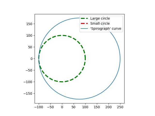
The plot shows large fixed circle drawn with a dashed line. The small circle is not visible because it is actually a single point. The ‘Spirograph’ curve is just a larger circle offset from the centre of the large circle.
If the small circle rolls around the larger circle without slipping, then the ratio of small circle to the large should be exactly in the ratio of the radius of the small circle to the radius of the large circle. So in this next image, the size of the small circle is 75, and the size of the large circle is 100. The smaller circle rotates 100/75 (4/3) times every time it goes around the large circle.

I’m going to finish up with a couple more images that look more like a standard ‘Spirograph’. The point P is still on the circumference of the smaller circle, but this makes little difference to the plots.

This show a typical curve that a ‘Spirograph’ would plot. The ‘mult2’ parameter controls how many lobes the figure has. In this case, with a value of 25, there should be 24 lobes.
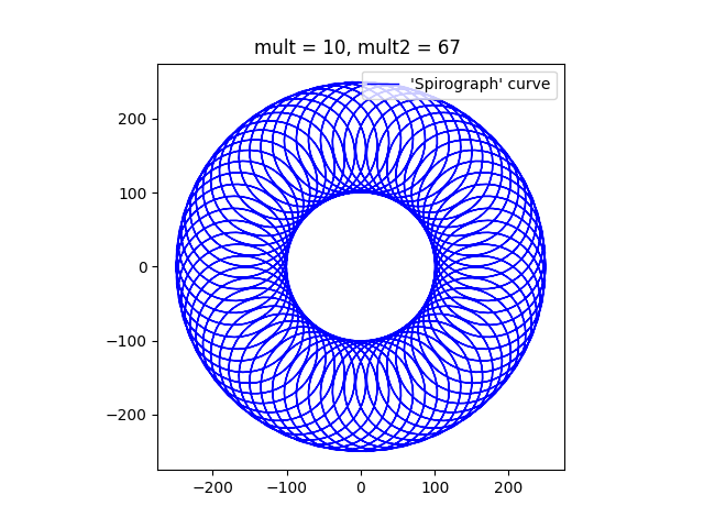
Finally, this image, with a mult2 value of 67 will have 66 lobes. When a Spirograph Wheel rotates around a fixed wheel, the pattern typically shows a rosette of loops, with a hole in the middle where the fixed wheel is located. I’m going to experiment with a moving wheel inside and if it is interesting I might do another post on the topic of ‘Spirographs’.
?Below I have pasted the program that I used to draw these images. Feel free to take it and alter it as much as you like.
import numpy as np
import matplotlib.pyplot as plt

# Dimensions of two circles
r1 = 100
r2 = 75
# c0 = [0,0]
# c1 = [1,0]

# Multipliers
mult = 10
mult2 = 67  # was 11

ax = plt.subplot()
ax.set_aspect( 1 )

# Parametric array for the larger circle
t1 = np.linspace(-2 * np.pi, 2 * np.pi, mult * 360)
# Parametric array for the smaller circle
t2 = t1 * mult2

# Calculation of X/y coordinates using the parametric arrays.
# x0 and y0 are the coordinates of the tangential point, B.
x0 = r1 * np.cos(t1)
y0 = r1 * np.sin(t1)
# plt.plot(x0, y0, label=("Large circle"), color = 'g', linewidth = 1, linestyle = '--')
# x1 and y1 are the cordinates of the centre of the small circle, C.
x1 = (r1 + r2) * np.cos(t1)
y1 = (r1 + r2) * np.sin(t1)
# x1a and y1a are the coordinates of D relative to C.
x1a = r2 * np.cos(t2)
y1a = r2 * np.sin(t2)
# plt.plot(x1a, y1a, label=("Small circle"), c = 'r', linewidth = 3, linestyle = '--')
# x2 and y2 are the coordinates of the desired point on the curve, D.

x2 = r2 * np.cos(t2)
y2 = r2 * np.sin(t2)

# Plot the Curve
# plt.plot(x1 - 1.5 * x2, y1 - 1.5 * y2)
plt.plot(x1 + x2, y1 + y2, label=("'Spirograph' curve"), c = 'b', linewidth = 1)

plt.title("mult = {}, mult2 = {} ".format(mult, mult2))
plt.legend(loc="upper right")
plt.show()