Sine – Me on the net

Plotting with ‘matplotlib’

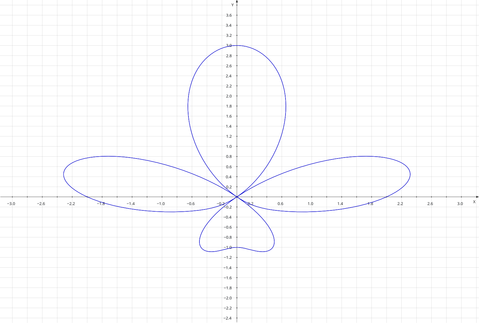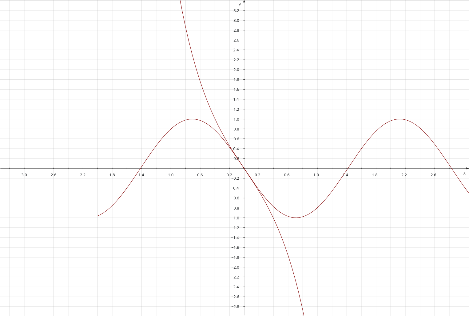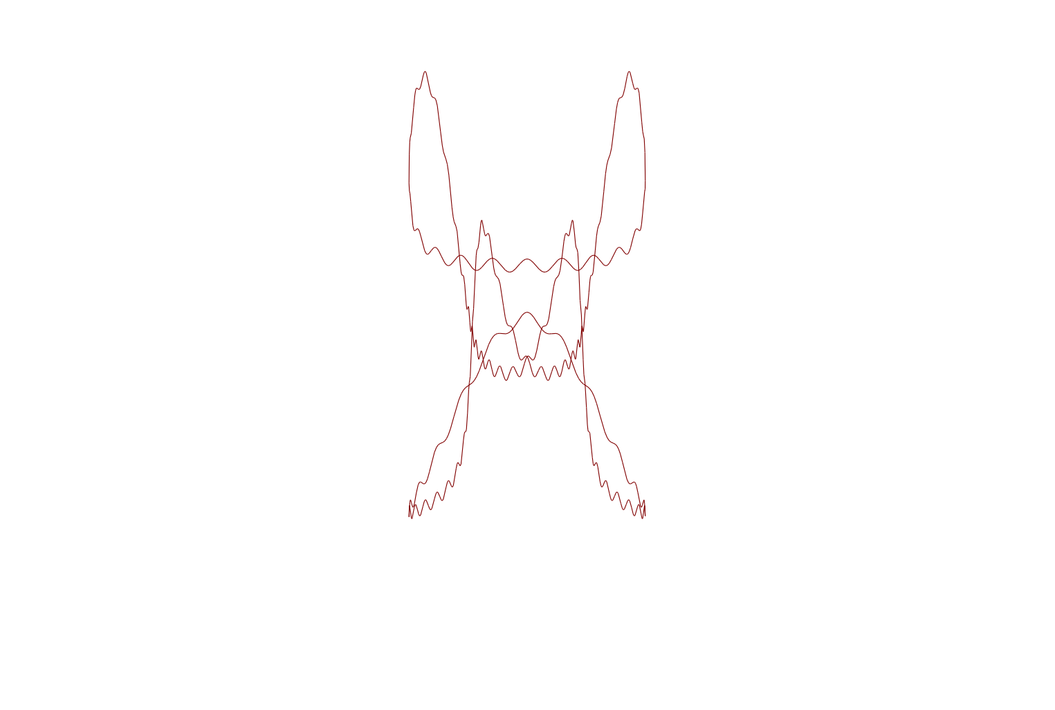
What is ‘matplotlib’? It’s a Python package which can be used to plot everything from a simple parabola or sine wave right up to complex statistical data. Of course, I use it just to print interesting curves, like the one above. I’ll discuss the program I wrote below.

Since it is a Python package it helps if you know how to write Python programs, but I don’t dive too deep into Python. Anyway, the above curves were printed by a program that is only eleven lines long!

At the top of the Python code, we need to tell it to use ‘matplotlib’ and I’ve included a line to tell the code that we need to use the ‘numpy’ maths package. Here’s the first bit of the program:

import matplotlib.pyplot as plt  # This is the plotting library
import numpy as np               # A common Python package

Plotting something involves matching one set of data against another. Commonly these sets of data are named ‘x’ and ‘y’, but they can have any names that the plotter desires. The relevant code in this program is as follows:

max_range = 1000
x = np.linspace(-2*np.pi, 2*np.pi, max_range)
y = np.sin(x)

The line that starts ‘x =’ uses the numpy ‘linspace’ routine to generate a numpy array of one thousand (max_range) elements evenly spaced between -2 time pi and 2 times pi. The line that starts ‘y =’ then creates another numpy array, taking the individual elements of the array x, applying the numpy sine function and appending the result to the end of the array y.

In the earliest version of this program, I created the two numpy arrays by means of a loop, but by creating numpy arrays using this method, I can do it in two lines. Like all good ideas I got it from someone else’s program on the Internet. There is only one program, the old joke goes, and that is the “Hello World!” program, and all other programs are descendants of that single archetype.

OK, so, I created two more arrays using the same technique, and here are the two lines of code:

z = np.sin(2*x)
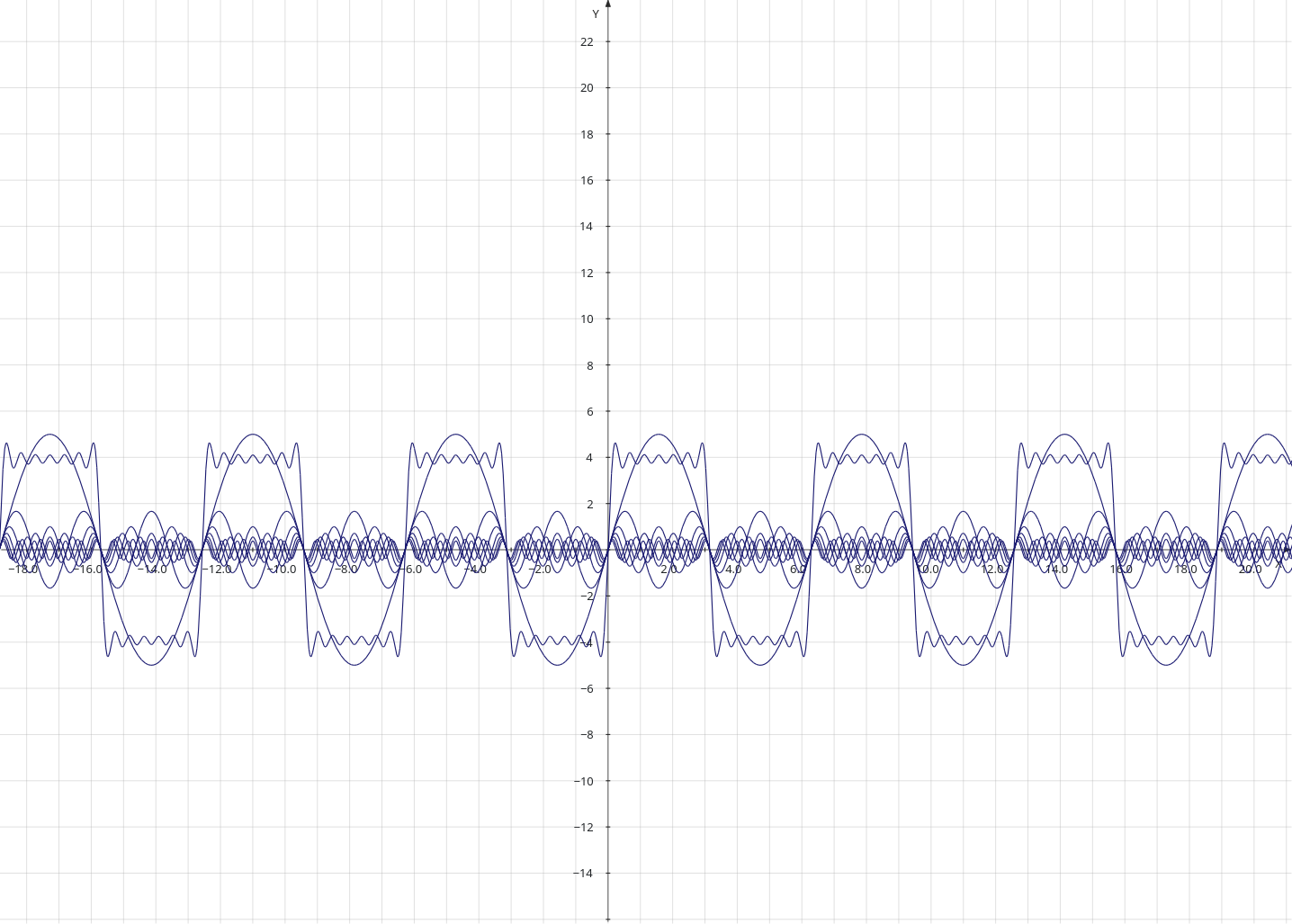
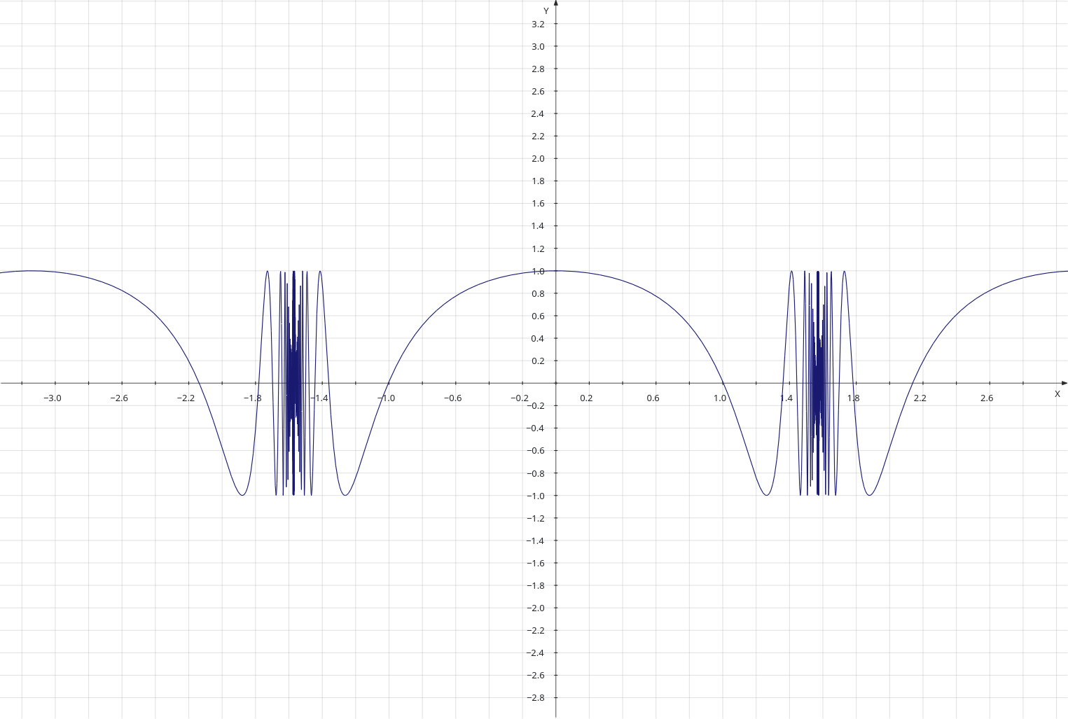
zz = np.sin(4*x)

So, I could have drawn three plots, one for each array, but that wouldn’t have been that interesting, so I decide to plot the sum of all three arrays (against the x array), and also the product of all three arrays (again, against the x array). Numpy arrays make this easy.

# y = np.sin(x) * np.sin(2*x) * np.sin(4*x)
plt.plot(x, y * z * zz, label='product')
# y = np.sin(x) + np.sin(2*x) + np.sin(4*x)
plt.plot(x, y + z + zz, label='sum')

The ‘plot’ statements each draw a line in the final figure, and generate a label for the line. The comments describe the curve in an x/y format, in a simple mathematical style .

The final couple of lines (see below) are needed to show the labels and the complete figure. Below is the whole Python program, comments and all.

import matplotlib.pyplot as plt
import numpy as np

# Basic Figures
# sine wave
max_range = 1000
x = np.linspace(-2*np.pi, 2*np.pi, max_range)
y = np.sin(x)

# sine wave, freq * 2
# x = np.linspace(-2*np.pi, 2*np.pi, max_range)
z = np.sin(2*x)
zz = np.sin(4*x)

# y = np.sin(x) * np.sin(2*x) * np.sin(4*x)
plt.plot(x, y * z * zz, label='product')
# y = np.sin(x) + np.sin(2*x) + np.sin(4*x)
plt.plot(x, y + z + zz, label='sum')

plt.legend()
plt.show()

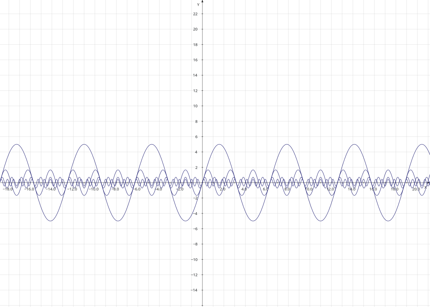
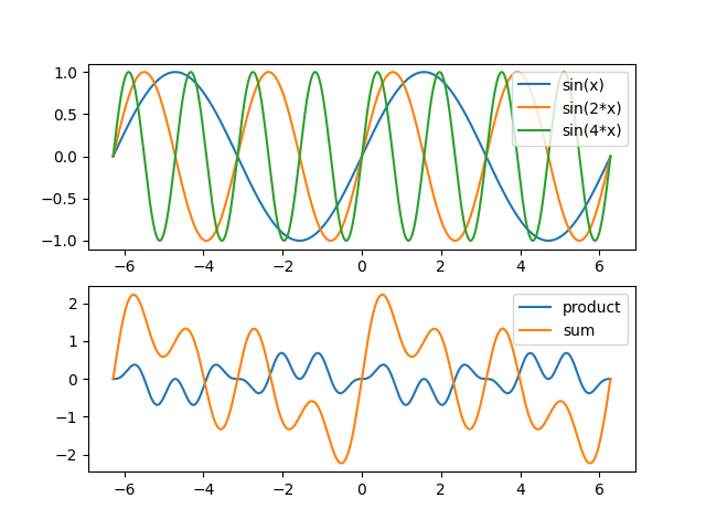
To close the post, I’m going present a more complex example. This one combines the plots described above, with a separate subplot of the three waves that were used to create the first subplot. At the very end is the source code.

import matplotlib.pyplot as plt
import numpy as np

# Basic Figures
# sine wave
max_range = 1000

fig, (ax1, ax2) = plt.subplots(2, 1)

# The x array runs from -2*pi to +2*pi
x = np.linspace(-2*np.pi, 2*np.pi, max_range)

# One component of the final plot
y = np.sin(x)

# sine wave, freq * 2
z = np.sin(2*x)
# Freq * 4
zz = np.sin(4*x)import matplotlib.pyplot as plt
import numpy as np

# Basic Figures
# sine wave
max_range = 1000

fig, (ax1, ax2) = plt.subplots(2, 1)

# The x array runs from -2*pi to +2*pi
x = np.linspace(-2*np.pi, 2*np.pi, max_range)

# One component of the final plot
y = np.sin(x)

# sine wave, freq * 2
z = np.sin(2*x)
# Freq * 4
zz = np.sin(4*x)
ax1.plot(x, y, label='sin(x)')
ax1.plot(x, z, label='sin(2*x)')
ax1.plot(x, zz, label='sin(4*x)')

legend1 = ax1.legend()

# y = sin(x) * sin(2x) * sin(4x)
ax2.plot(x, y * z * zz, label='product')
# y = sin(x) + sin(2x) + sin(4x)
ax2.plot(x, y + z + zz, label='sum')

legend2 = ax2.legend()

plt.show()
ax1.plot(x, y, label='sin(x)')
ax1.plot(x, z, label='sin(2*x)')
ax1.plot(x, zz, label='sin(4*x)')

legend1 = ax1.legend()

# y = sin(x) * sin(2x) * sin(4x)
ax2.plot(x, y * z * zz, label='product')
# y = sin(x) + sin(2x) + sin(4x)
ax2.plot(x, y + z + zz, label='sum')

legend2 = ax2.legend()

plt.show()

A Simple KmPlot Example

A simple sine wave is not that interesting. However adding sine waves together can produce something more aesthetically satisfying. I could, for example, add another sine wave with a higher frequency to the above simple sine wave, as shown below.

The above diagram shows the result of adding a sine wave of three times the original frequency to the first wave. Below I show the result of adding a third sine wave of five times the original fequency to the first.

A pattern is beginning to emerge from this process. I’ll add a few more terms to the summation.

This shows the sum of the terms up to the the term for the sine wave which is 13 times the original frequency. Those who have done some maths probably recognise that this is tending towards a square wave. Here’s a link to a MatLab version of what I’ve done here.

Here’s a depiction of all the individual waves that have been added together, plus the final result.

Here’s an image of just a few of the waves. It’s probably more aesthetic than the full set!

A couple of times when I was creating the above series of plots, I made mistakes, and ended up with some more interesting graphs, but I discarded those ‘mistakes’ and stuck closely to my original idea, which was to show how simply adding a few sine waves together could result in an approximate square wave.

In fact the Fourier series for a square wave can be expressed as an infinite sum of sine waves, as shown here. A fairly complex mathematical fact can be approximated by a few simple plots.

Now I’m going to go back to the ‘mistakes’ that I made and rejected earlier when developing and writing this post.

Plotting using KmPlot

I created the above image using a program called ‘KmPlot’. It is a program for the KDE desktop for plotting mathematical functions. The function that I used for the above is something like the following:-

2∙cos(y) + 1.5∙sin(3y) = cos(5x)  −0.5∙sin(9x)

I don’t plot these curves for scientific or mathematical reasons, and that is why I can’t be 100% sure of which function(s) I actually used. I plot these curves simply to create shapes and designs which I find attractive.

I continually tweak the equations that I use until I find something that I like. There is an endless array of possibilities, even with very similar equations and for example the following image:-

The equation in this case is:-

k(x) = tan(tan(x))

The two plots above use trigonometric functions, exponential function can produce some interesting images, too, like this one:-

The equation of this curve is simply:-

s(x) = 1/x−1/x^3+1/x^5−1/x^7+1/^9

I just fiddle with these equations to produce new images. For instance, the above equation has alternating terms. What would happen if I changed all the negative terms to positive ones. This is the answer to that question:-

It is similar but different. The equation is as follows:-

s(x) = 1/x+1/x^3+1/x^5+1/x^7+1/^9

Just adding sine and cosine terms together sometimes produces interesting results. Here’s one:-

In the case of these curves, the main function is made up of multiple smaller functions, so I can’t post the formula, unfortunately. A few simple curves plotted on the same plot can produce interesting images. Below is a plot of four curves of the hyperbolic trig functions, sinh and cosh. It demonstrates how an interesting image can be built up from several curves:-

At the time I created that I was trying to recreate the following image. I have the image, but I don’t have the source! It is long gone:-

Just by fiddling with the functions and adding and multiplying them together can serendipitously result in interesting images. Here’s one. I don’t recall how I created it:-

My penultimate image is the result of trying to re-create the above image. It resembles a drawing of a flying creature, and results from lucky mistakes in copying the equations:-

That’s it for now. KmPlot allows you to create simple or complex shapes using only a little bit of elementary maths. Just by fiddling with the equations you can create weird and interesting images and I for one can’t predict what I am going to create!

Here’s one last image. This one is different from most of the others, but it has a pleasing stretched and compressed feel to it:-