More ‘Spirograph (®) plots using ‘matplotlib’

‘Spirograph’ includes toothed rings which can be used with small disks to draw Spirograph patterns inside the ring. The small toothed rolls around the inside of the fixed ring, producing the typical Spirograph spirals.

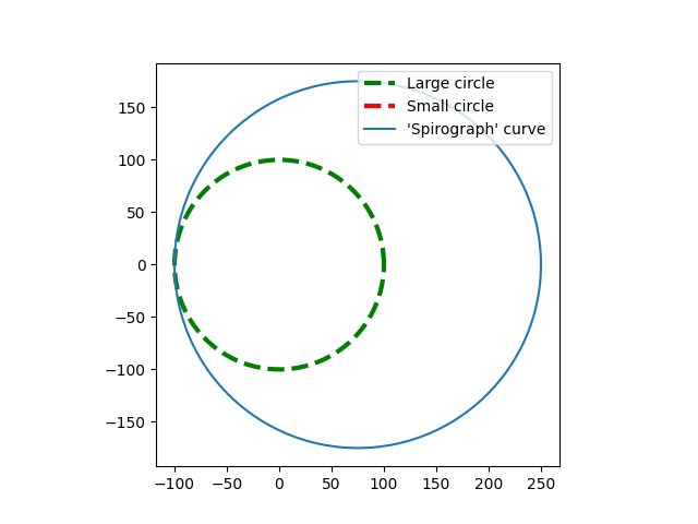
The diagram above shows how this works. The small circle rolls around inside the larger circle (which represents the inside of the ring). If there is no slippage, the small circle rotates in the opposite direction to its movement around the larger circle.

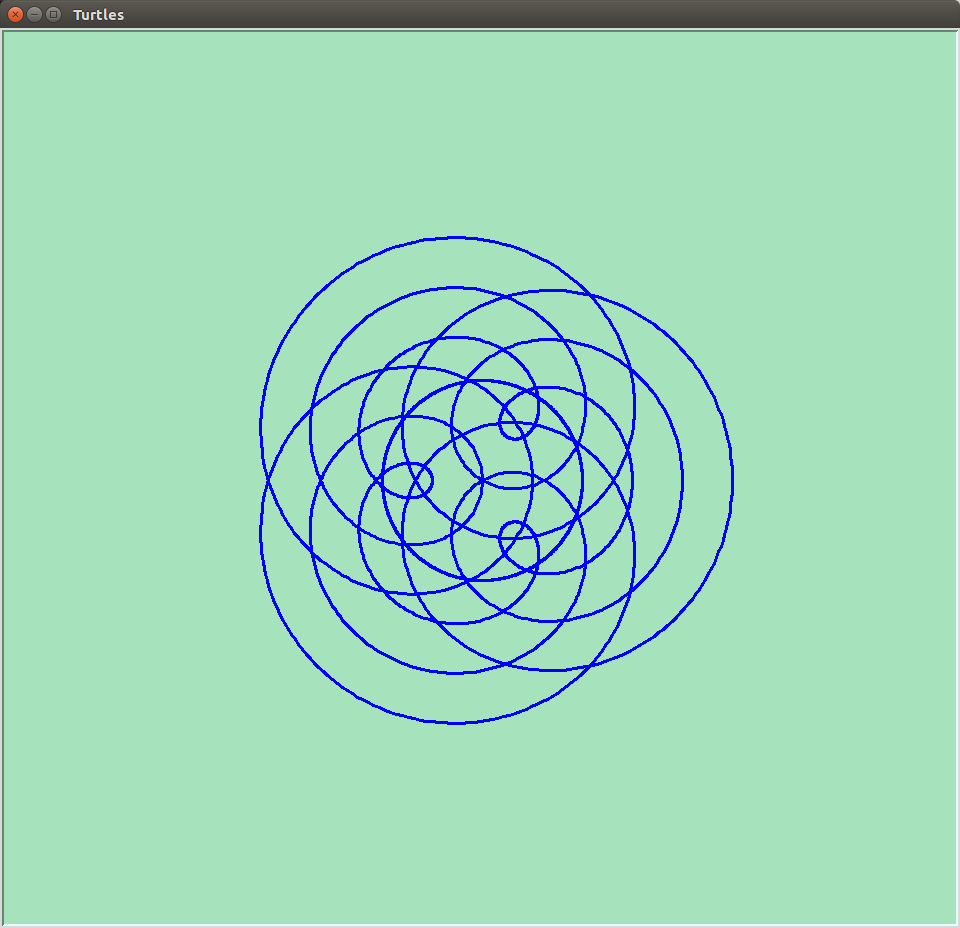
I modified my Python program to simulate this situation. As before, the rate of rotation of the smaller circle can be controlled by varying the ‘mult2’ variable in the program. To start with I used a small value for the variable as shown below.

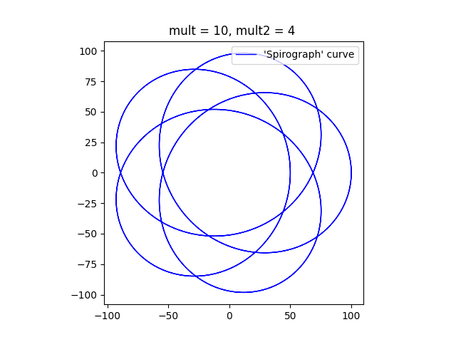
The diagram has five ‘lobes’ and an empty patch in the middle. The curve can never go through the centre. If the ratio of the sizes of the circles is less than one half, then smaller circle is not big enough to reach the centre of the larger circle. If the ratio of the sizes of the circles is greater than one half, then the point on the circumference of the smaller circle that is drawing the curve (point D on the diagram above) never falls on the centre of the larger circle. If the ratio of sizes is exactly one half, all the loops will pass through the centre of the larger circle.

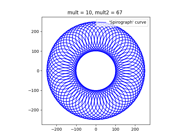
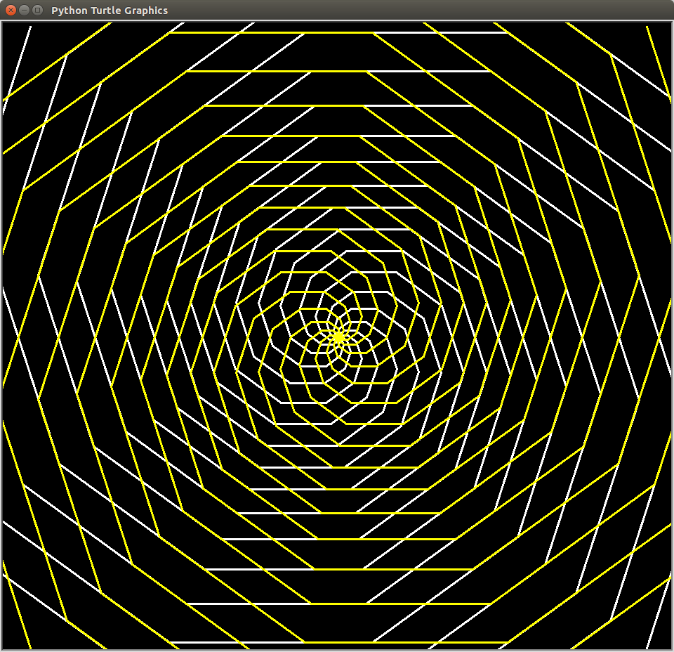
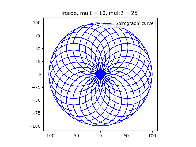
As the multiplier ‘mult2’ is increased, the curve comes to resemble the circular shape of a typical Spirograph. I think that it looks a bit like a torus or a donut.

I’m not going to try to emulate the behaviour of the non-circular Spirograph components. In fact, I have only emulated the circular ones, but not completely. I’ve only plotted the curves that would result if the point P (the pen) corresponded to the point D (on the smaller circle) in the diagram above.

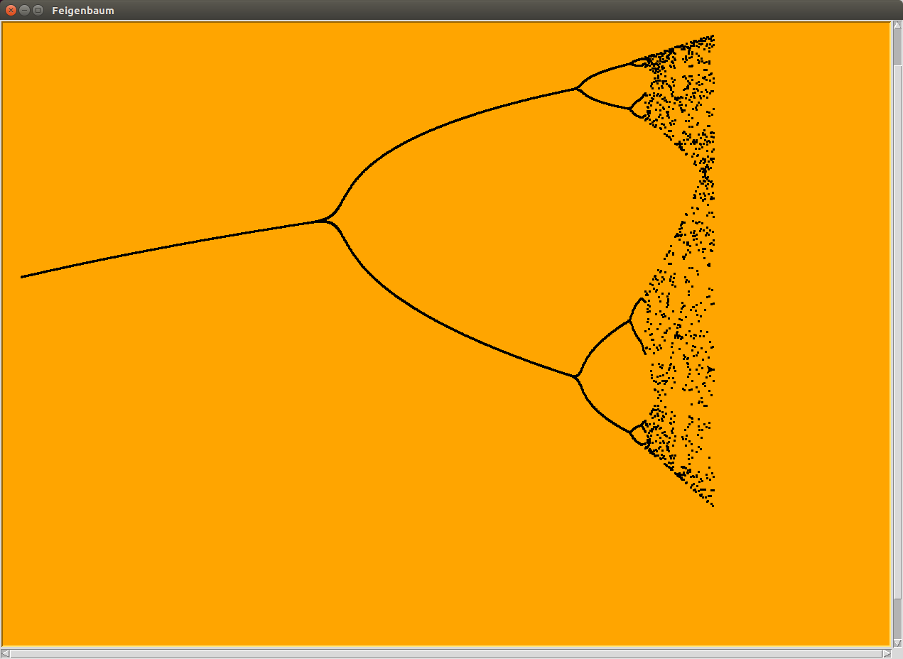
Here’s one final plot, where the ratio of the smaller circle to the larger circle is exactly one half. The program draws a pleasant chrysanthemum or dahlia shape.

Finally, here’s the Python program that I used to draw these diagrams. To get the different figures, I’ve changed the multipliers, mainly ‘mult2’. I’ve also changed the sizes of the circles (variables ‘large’ and ‘small’) to get some of them.


import numpy as np
import matplotlib.pyplot as plt

# Dimensions of two circles
r1 = 100
r2 = 50
# c0 = [0,0]
# c1 = [1,0]

# Multipliers
mult = 10   # Used to generate the number of points plotted.
mult2 = 25  # Controls speed of rotation of the smaller circle, relative to the first.

ax = plt.subplot()
ax.set_aspect( 1 )

# Parametric array for the larger circle
t1 = np.linspace(-2 * np.pi, 2 * np.pi, mult * 360)
# Parametric array for the smaller circle
t2 = t1 * mult2

# Calculation of X/y cordinates using the parametric arrays.
# x0 and y0 are the coordinates of the tangential point, B.
x0 = r1 * np.cos(t1)
y0 = r1 * np.sin(t1)
# plt.plot(x0, y0, label=("Large circle"), color = 'r', linewidth = 2, linestyle = '--')
# x1 and y1 are the cordinates of the centre of the small circle, C.
x1 = (r1 - r2) * np.cos(t1)
y1 = (r1 - r2) * np.sin(t1)
# x1a and y1a are the coordinates of D relative to C.
x1a = r2 * np.cos(t2)
y1a = r2 * np.sin(t2)
# plt.plot(x1a, y1a, label=("Small circle"), c = 'r', linewidth = 2, linestyle = '--')
# x2 and y2 are the coordinates of the desired point on the curve, D.
plt.plot(x0[0],y0[0], color='r')
# The small circle rolls in the opposite direction if it is inside
x2 = r2 * np.cos(-t2)
y2 = r2 * np.sin(-t2)

# Plot the Curve
# plt.plot(x1 - 1.5 * x2, y1 - 1.5 * y2)
plt.plot(x1 + x2, y1 + y2, label=("'Spirograph' curve"), c = 'b', linewidth = 1)

plt.title("Inside, mult = {}, mult2 = {} ".format(mult, mult2))
plt.legend(loc="upper right")
plt.show()

Drawing ‘Spirograph'(®)-like Curves with matplotlib

‘Spirograph’® is a set of devices which can be used to draw some interesting looping curves. It consists of various toothed wheels and other toothed shapes with small holes them. A wheel or other shape is chosen, and fixed to the drawing surface. A second wheel is placed so that its teeth interlock with the teeth on the second wheel and a pen is inserted into a hole in the second wheel. The pen is moved to keep the two gear wheels enmeshed at all times. As a result the pen traces out a curve.

This can, of course, be plotted mathematically, using a tool like ‘matplotlib’. The above diagram shows how the Spirograph system works. The circle representing the first wheel is centred on point A and is fixed. The other circle is centred on point C, rolls around the first circle, and is always in contact with the first circle at point B. The point P is a point inside the smaller circle, and the line CD is the radius which passes through point B.

It is easy to see that the centre of the smaller circle (C) travels in a larger circle around the static circle. This larger circle (not drawn) has a radius is equal to the sum of the radii of the two circles. This radius corresponds to the line AC. As C travels around the circle, the smaller circle, CD, rotates. Meanwhile, the point P on CD traces out the curve we are interested in.

In the ‘Spirograph’ case, the two circles are linked by the teeth on the gears wheels. This connection ensures that the smaller circle rotates at a fixed speed. The Wikipedia page on the ‘Spirograph’ system mentions that the teeth prevent any slipping.

In the program generated case, smaller wheel can be programmed to rotate at any rate that is desired, with ‘slippage’. It can, for example, be programmed to move around the large circle without rotating at all. The next image shows what happens then. [Note: For simplicity, the point P is assumed to be located on the circumference of the small circle.]

The plot shows large fixed circle drawn with a dashed line. The small circle is not visible because it is actually a single point. The ‘Spirograph’ curve is just a larger circle offset from the centre of the large circle.

If the small circle rolls around the larger circle without slipping, then the ratio of small circle to the large should be exactly in the ratio of the radius of the small circle to the radius of the large circle. So in this next image, the size of the small circle is 75, and the size of the large circle is 100. The smaller circle rotates 100/75 (4/3) times every time it goes around the large circle.

I’m going to finish up with a couple more images that look more like a standard ‘Spirograph’. The point P is still on the circumference of the smaller circle, but this makes little difference to the plots.

This show a typical curve that a ‘Spirograph’ would plot. The ‘mult2’ parameter controls how many lobes the figure has. In this case, with a value of 25, there should be 24 lobes.

Finally, this image, with a mult2 value of 67 will have 66 lobes. When a Spirograph Wheel rotates around a fixed wheel, the pattern typically shows a rosette of loops, with a hole in the middle where the fixed wheel is located. I’m going to experiment with a moving wheel inside and if it is interesting I might do another post on the topic of ‘Spirographs’.

?Below I have pasted the program that I used to draw these images. Feel free to take it and alter it as much as you like.

import numpy as np
import matplotlib.pyplot as plt

# Dimensions of two circles
r1 = 100
r2 = 75
# c0 = [0,0]
# c1 = [1,0]

# Multipliers
mult = 10
mult2 = 67  # was 11

ax = plt.subplot()
ax.set_aspect( 1 )

# Parametric array for the larger circle
t1 = np.linspace(-2 * np.pi, 2 * np.pi, mult * 360)
# Parametric array for the smaller circle
t2 = t1 * mult2

# Calculation of X/y coordinates using the parametric arrays.
# x0 and y0 are the coordinates of the tangential point, B.
x0 = r1 * np.cos(t1)
y0 = r1 * np.sin(t1)
# plt.plot(x0, y0, label=("Large circle"), color = 'g', linewidth = 1, linestyle = '--')
# x1 and y1 are the cordinates of the centre of the small circle, C.
x1 = (r1 + r2) * np.cos(t1)
y1 = (r1 + r2) * np.sin(t1)
# x1a and y1a are the coordinates of D relative to C.
x1a = r2 * np.cos(t2)
y1a = r2 * np.sin(t2)
# plt.plot(x1a, y1a, label=("Small circle"), c = 'r', linewidth = 3, linestyle = '--')
# x2 and y2 are the coordinates of the desired point on the curve, D.

x2 = r2 * np.cos(t2)
y2 = r2 * np.sin(t2)

# Plot the Curve
# plt.plot(x1 - 1.5 * x2, y1 - 1.5 * y2)
plt.plot(x1 + x2, y1 + y2, label=("'Spirograph' curve"), c = 'b', linewidth = 1)

plt.title("mult = {}, mult2 = {} ".format(mult, mult2))
plt.legend(loc="upper right")
plt.show()

Turtles and More

Kina
Turtle graphics. This to me resembles a Kina or Sea Urchin

My wife recently became interested in the Spirograph (™) system. Since her birthday was coming up, so did I, for obvious reasons. If you have never come across Spirograph (™) I can highly recommend it, as it enables the production of glorious swirls and spirals, using a system of toothed wheels and other shapes. When you use multicoloured pen, the results can be amazing.

Of course, I had to translate this interest into the computer sphere, and I immediately recalled “Turtle Graphics” which I have used before. It is possible to create graphics very similar to the Spirograph (™) designs very simply with Turtle Graphics.

Trefoil
This resembles the sort of things generated by Spirograph (TM)

Turtle Graphics have a long history, stretching back at least to the educational programming language Logo. Although variations of the original Logo language exist, they are fairly rare, but the concept of Turtle Graphics, where a cursor (sometimes shown as the image of a cartoon turtle) draws a line on a page, still exists. The turtle can be directed to move in a particular way, based on instructions by the programmer.

For instance the turtle can be instructed to move forward a certain distance, turn right through 90°, and repeat this process three times. The result is a small square. Or the turtle could be instructed to move forward and turn only 60°, repeating this 5 times to draw a hexagon. Using simple instructions like this allow the drawing of practically anything.

Square and Hexagonal spirals
Square and hexagonal spirals drawn by Turtle Graphics

I use an implementation of Turtle Graphics in the turtle module of the Python programming language but it is probably available for other programming languages. Python is probably an easy language to learn from scratch than Logo, and in addition Python can be used for many other things than Turtle Graphics. Python is available for Windows, OS/X, and Linux/Unix, and for several other older or less well known platforms.

Where things become interesting is when the looping abilities of Python are used to enhance a program. If the programmer gets the turtle to draw a square, then makes the turtle turn a little and repeats the process, the result is a circular pattern. Starting with a more interesting shape can produce some interesting patterns.

Rotated Square - Turtle graphics
Rotated Square – Turtle graphics

After a while, though, the patterns begin to seem very similar to one another. One way to add a bit of variation is to use the ability to make the turtle move to a specific position, drawing a line on the way. As an example, consider a stick hinged to another stick, much like a nunchaku. If one stick rotates as a constant speed and the second stick rotates at some multiple of that, then the end of the second stick traces out a complex curve.

Flower shape
Flower shape – turtle graphics

In Python this can be expressed like this:

x = int(a * math.sin(math.radians(c * i)) + b * math.sin(math.radians(d * i)))
y = int(a * math.cos(math.radians(c * i)) + b * math.cos(math.radians(d * i)))

where c and d are the rates of rotation of the two sticks and and b are the lengths of the stick. i is a counter that causes the two sticks to rotate. If the turtle is moved to the position x, y, a line is drawn from the previous position, and a curve is drawn.

The fun part is varying the various parameters, a, b, c, d, to see what effect that has. The type of curve that is created here is an epicycloid. For larger values of c and d the curves resemble the familiar shapes generated by Spirograph (™).

Epitrochoids
Epitrochoids

The equations above use the same constants in each equation. If the constant are different, some very interesting shapes appear, but I’m not going to go into that here. Suffice it to say, I got distracted from writing this post by playing around with those constants!

The above equations do tend to produce curves with radial symmetry, but there is another method that can be used to produce other curves, this time with rotational symmetry. For instance, a curve can be generated by moving to new point depending on the latest move. This process is then iterative.

Gravity Wave - turtle graphics
Gravity Wave turtle graphics

For instance, the next position could be determined by turning through an angle and move forward a little more than the last time. Something like this snippet of code would do that:

for i in range(1, 200):
t.forward(a)
t.pendown()

t.left(c)
a = a + 1
c = c + 10

This brings up a point of interest. If you run code like this, ensure that you don’t stop it too soon. This code causes the turtle to spin and draw in a small area for a while, and then fly off. However it quickly starts to spin again in a relatively small area before once more shooting off again. Evidently it repeats this process as it continues to move off in a particular direction.

Turtle graphics - a complex curve from a simple equation
Turtle graphics – a complex curve from a simple equation

Another use of turtle graphics is to draw graphs of functions, much like we learnt to do in school with pencil and squared paper. One such function is the cycloid function:

x = r(t – sine(t))

y = r(1 – cosine))

This function describes the motion of a wheel rolling along a level surface and can easily be translated into Python. More generally it is the equation of a radius of a circle rolling along a straight line. If a different point is picked, such a point on a radius inside the circle or a point outside the circle on the radius extended, a family of curves can be generated.

Cycloid curve - turtle graphics
Cycloid curve – turtle graphics

Finally, a really technical example. An equation like the following is called a dynamic equation. Each new ‘x’ is generated from the equation using the previous ‘x’. If this process is repeated many times, then depending on the value of ‘r’, the new value of ‘x’ may become ever closer to the previous value of ‘x’.

x(n+1) = rx(n)(1 – x(n))

If the value of ‘r’ is bigger than a certain value and less than another value, then ‘x’ flip-flops between two values. If the value of ‘r’ is bigger than the other value, and smaller than yet another value then ‘x’ rotates between 4 values. This doubling happens again and again in a “period doubling cascade“.

Turtle graphics - electron orbitals
Turtle graphics – electron orbitals

I’ve written a turtle program to demonstrate this. First a value for ‘r’ is chosen, then the equation is repeated applied 1,000 times, and the next 100 results are plotted, x against r. In the end result, the period doubling can easily be seen, although after a few doubling, the results become messy (which may be related to the accuracy and validity of my equations, and the various conversion between float and integer types).

Period doubling
The “fig tree” curve calculated in Python and plotted by Turtle Graphics.